Pandas Tips Collection

Pandas Tips Collection#

このノートブックでは、Pandasを使ったデータ分析をさらに効率化するための便利な関数やメソッドを紹介します。
基礎的な操作は把握している方向けの内容で、知っていると役立つ、作業が効率化できるようなテクニックや便利な関数をまとめています。
お役に立てば幸いです！

基本的に章ごとに独立して実行できるようにしてあります
目次の内容を見て、気になるものから見ても大丈夫です！

基本的にDataFrameのメソッドはDataFrameのコピーを返す#

DataFrameの各種メソッドは基本的にDataFrameのコピーを返すので、元のDataFrameは何も変わらないです。
もとのDataFrameにメソッドを適用したい場合は、2通りやり方があります

inplaceオプションをTrueにする（例：df.reset_index(inplace=True)
元の変数にメソッドを適用した変数を代入する（例：df = df.reset_index()）

inplaceオプションを使った方が、メモリ効率は良いみたいです。
（inplaceオプションが無いメソッドもあります）

# # やり方①
# # inplace=Trueと設定する
# df.reset_index(inplace=True)

# # やり方②
# # 元の変数にメソッドを適用した変数を代入
# df = df.reset_index()

import plotly.express as px
df = px.data.iris()

# オプションを何も指定しないでメソッド(例えばreset_index)を実行
df.reset_index() # メソッドが適用されたオブジェクトが返される（ここでは表示されるだけ）

	index	sepal_length	sepal_width	petal_length	petal_width	species	species_id
0	0	5.1	3.5	1.4	0.2	setosa	1
1	1	4.9	3.0	1.4	0.2	setosa	1
2	2	4.7	3.2	1.3	0.2	setosa	1
3	3	4.6	3.1	1.5	0.2	setosa	1
4	4	5.0	3.6	1.4	0.2	setosa	1
...	...	...	...	...	...	...	...
145	145	6.7	3.0	5.2	2.3	virginica	3
146	146	6.3	2.5	5.0	1.9	virginica	3
147	147	6.5	3.0	5.2	2.0	virginica	3
148	148	6.2	3.4	5.4	2.3	virginica	3
149	149	5.9	3.0	5.1	1.8	virginica	3

150 rows × 7 columns

# 元のDataFrameは何も変わらない
df

	sepal_length	sepal_width	petal_length	petal_width	species	species_id
0	5.1	3.5	1.4	0.2	setosa	1
1	4.9	3.0	1.4	0.2	setosa	1
2	4.7	3.2	1.3	0.2	setosa	1
3	4.6	3.1	1.5	0.2	setosa	1
4	5.0	3.6	1.4	0.2	setosa	1
...	...	...	...	...	...	...
145	6.7	3.0	5.2	2.3	virginica	3
146	6.3	2.5	5.0	1.9	virginica	3
147	6.5	3.0	5.2	2.0	virginica	3
148	6.2	3.4	5.4	2.3	virginica	3
149	5.9	3.0	5.1	1.8	virginica	3

150 rows × 6 columns

# 元のデータフレームを書き換えるやり方　その１
# inplaceオプションをTrueに設定
df.reset_index(inplace=True)

df

	index	sepal_length	sepal_width	petal_length	petal_width	species	species_id
0	0	5.1	3.5	1.4	0.2	setosa	1
1	1	4.9	3.0	1.4	0.2	setosa	1
2	2	4.7	3.2	1.3	0.2	setosa	1
3	3	4.6	3.1	1.5	0.2	setosa	1
4	4	5.0	3.6	1.4	0.2	setosa	1
...	...	...	...	...	...	...	...
145	145	6.7	3.0	5.2	2.3	virginica	3
146	146	6.3	2.5	5.0	1.9	virginica	3
147	147	6.5	3.0	5.2	2.0	virginica	3
148	148	6.2	3.4	5.4	2.3	virginica	3
149	149	5.9	3.0	5.1	1.8	virginica	3

150 rows × 7 columns

# サンプルデータ再取得
df = px.data.iris()

# 元のデータフレームを書き換えるやり方　その２
# 元の変数に代入
df = df.reset_index()

# メソッドが適用されている
df

	index	sepal_length	sepal_width	petal_length	petal_width	species	species_id
0	0	5.1	3.5	1.4	0.2	setosa	1
1	1	4.9	3.0	1.4	0.2	setosa	1
2	2	4.7	3.2	1.3	0.2	setosa	1
3	3	4.6	3.1	1.5	0.2	setosa	1
4	4	5.0	3.6	1.4	0.2	setosa	1
...	...	...	...	...	...	...	...
145	145	6.7	3.0	5.2	2.3	virginica	3
146	146	6.3	2.5	5.0	1.9	virginica	3
147	147	6.5	3.0	5.2	2.0	virginica	3
148	148	6.2	3.4	5.4	2.3	virginica	3
149	149	5.9	3.0	5.1	1.8	virginica	3

150 rows × 7 columns

メソッドチェーン：きれいにコードが書ける#

Pythonでは、( )でくくると中で自由に改行できます。逆に( )でくくらず改行したい場合は毎回「\」 (環境によっては円マーク)を書く必要があります。

pandasでよく使いますが、( )でくくってピリオドの直前で改行するのが楽で見栄えもよいと思います。

import pandas as pd
import seaborn as sns
df = sns.load_dataset("titanic")

# ()でくくる場合、自由に改行可能
df_agg = (
    df.groupby(["sex","alive"])
    .size()
    .rename("count")
    .reset_index()
)

# ()でくくらない場合 \(バックスラッシュ)を都度つける必要がある
df_agg = \
    df.groupby(["sex","alive"])  \
    .size()  \
    .rename("count")  \
    .reset_index()

query：簡単な条件指定方法#

queryメソッドを使うと、楽な書き方で条件指定できて便利です。 (ただし、処理速度は基本的な条件指定の仕方に劣るみたいです)

https://pandas.pydata.org/docs/reference/api/pandas.DataFrame.query.html

import pandas as pd
import seaborn as sns

df = sns.load_dataset('iris') # サンプルデータ

# 基本的な条件指定の仕方
df[(df["species"]=="setosa")&(df["sepal_width"]<3)]

	sepal_length	sepal_width	petal_length	petal_width	species
8	4.4	2.9	1.4	0.2	setosa
41	4.5	2.3	1.3	0.3	setosa

# queryを使った条件指定の仕方
df.query("species=='setosa' and sepal_width<3")

	sepal_length	sepal_width	petal_length	petal_width	species
8	4.4	2.9	1.4	0.2	setosa
41	4.5	2.3	1.3	0.3	setosa

display：表示方法の調整#

pd.options.display.max_rowsでdisplay時の最大表示行数を恒久的に変更できますが、一時的に表示行数増やしたいということがあるはず

そんな時はpd.option_contextが便利です💡 関数化しておくと使いやすいです

こちらの記事がわかりやすいです https://note.nkmk.me/python-pandas-option-display/

公式ドキュメント
https://pandas.pydata.org/docs/user_guide/options.html

小数点以下の桁数: display.precision
有効数字（有効桁数）: display.float_format
最大表示行数: display.max_rows
最大表示列数: display.max_columns
省略時の行数・列数表示: display.show_dimensions
全体の最大表示幅: display.width
列ごとの最大表示幅: display.max_colwidth
列名表示の右寄せ・左寄せ: display.colheader_justify

import pandas as pd
import seaborn as sns
df = sns.load_dataset('iris') # サンプルデータ

df

	sepal_length	sepal_width	petal_length	petal_width	species
0	5.1	3.5	1.4	0.2	setosa
1	4.9	3.0	1.4	0.2	setosa
2	4.7	3.2	1.3	0.2	setosa
3	4.6	3.1	1.5	0.2	setosa
4	5.0	3.6	1.4	0.2	setosa
...	...	...	...	...	...
145	6.7	3.0	5.2	2.3	virginica
146	6.3	2.5	5.0	1.9	virginica
147	6.5	3.0	5.2	2.0	virginica
148	6.2	3.4	5.4	2.3	virginica
149	5.9	3.0	5.1	1.8	virginica

150 rows × 5 columns

# 恒久的に変更したい場合
pd.options.display.max_rows = 60
pd.options.display.max_columns = 3

# オプションリセット
pd.reset_option("all")

<ipython-input-18-6c2018863eb3>:2: FutureWarning: data_manager option is deprecated and will be removed in a future version. Only the BlockManager will be available.
  pd.reset_option("all")
<ipython-input-18-6c2018863eb3>:2: FutureWarning: use_inf_as_na option is deprecated and will be removed in a future version. Convert inf values to NaN before operating instead.
  pd.reset_option("all")

# 一時的に変更したい場合
def display_more(df,max_rows=1000,max_columns=100,max_colwidth=50,precision=6):
  option_tuple = (
      'display.max_rows',max_rows,
      'display.max_columns',max_columns,
      'display.max_colwidth',max_colwidth, # 文字数
      'display.precision',precision # 小数桁数
  )
  with pd.option_context(*option_tuple):
      display(df)

display_more(df,max_rows=20)

	sepal_length	sepal_width	petal_length	petal_width	species
0	5.1	3.5	1.4	0.2	setosa
1	4.9	3.0	1.4	0.2	setosa
2	4.7	3.2	1.3	0.2	setosa
3	4.6	3.1	1.5	0.2	setosa
4	5.0	3.6	1.4	0.2	setosa
...	...	...	...	...	...
145	6.7	3.0	5.2	2.3	virginica
146	6.3	2.5	5.0	1.9	virginica
147	6.5	3.0	5.2	2.0	virginica
148	6.2	3.4	5.4	2.3	virginica
149	5.9	3.0	5.1	1.8	virginica

150 rows × 5 columns

loc, iloc：範囲指定の注意点#

locとilocの範囲指定方法の違いに注意が必要です。

locではコロン右側で指定した値までの範囲が抽出されます
ilocではコロン右側で指定した番号の1個手前までの範囲が抽出されます

import pandas as pd
import seaborn as sns
df = sns.load_dataset('iris') # サンプルデータ

df.loc[0:4,"sepal_length":"petal_width"]

	sepal_length	sepal_width	petal_length	petal_width
0	5.1	3.5	1.4	0.2
1	4.9	3.0	1.4	0.2
2	4.7	3.2	1.3	0.2
3	4.6	3.1	1.5	0.2
4	5.0	3.6	1.4	0.2

df.iloc[0:4,0:3]

	sepal_length	sepal_width	petal_length
0	5.1	3.5	1.4
1	4.9	3.0	1.4
2	4.7	3.2	1.3
3	4.6	3.1	1.5

reindex：indexを再設定#

reindexを使うと、SeriesやDataFrameのindexを再設定できます！
任意の順番にindexを並び替えたいときや、新たなindexを追加したいときに便利です

詳細はこちらの記事が参考になります👇
https://note.nkmk.me/python-pandas-reindex/

import pandas as pd
s = pd.Series([0,3,6,12],index=[0,1,2,4],name='data')
s

	data
0	0
1	3
2	6
4	12

dtype: int64

# もとのデータにないindexも含め再設定
s = s.reindex([0,1,2,3,4])
s

	data
0	0.0
1	3.0
2	6.0
3	NaN
4	12.0

dtype: float64

info：メモリ使用量などがわかる#

DataFrameのinfoメソッドで、そのDataFrameのメモリ使用量や各列の欠損数と型をまとめて見ることができます。

import pandas as pd
import seaborn as sns
df = sns.load_dataset('iris') # サンプルデータ
df.info()

<class 'pandas.core.frame.DataFrame'>
RangeIndex: 150 entries, 0 to 149
Data columns (total 5 columns):
 #   Column        Non-Null Count  Dtype  
---  ------        --------------  -----  
 0   sepal_length  150 non-null    float64
 1   sepal_width   150 non-null    float64
 2   petal_length  150 non-null    float64
 3   petal_width   150 non-null    float64
 4   species       150 non-null    object 
dtypes: float64(4), object(1)
memory usage: 6.0+ KB

describe：基本統計#

DataFrameのdescribeメソッドで統計情報を出力できます。
includeオプションで、対象のカラムを選択でき、[object]と指定すると文字列カラムが対象となります。

公式ドキュメント https://pandas.pydata.org/docs/reference/api/pandas.DataFrame.describe.html

import pandas as pd
import seaborn as sns
df = sns.load_dataset('penguins') # サンプルデータ

df.describe() # 数値を持つカラム

	bill_length_mm	bill_depth_mm	flipper_length_mm	body_mass_g
count	342.000000	342.000000	342.000000	342.000000
mean	43.921930	17.151170	200.915205	4201.754386
std	5.459584	1.974793	14.061714	801.954536
min	32.100000	13.100000	172.000000	2700.000000
25%	39.225000	15.600000	190.000000	3550.000000
50%	44.450000	17.300000	197.000000	4050.000000
75%	48.500000	18.700000	213.000000	4750.000000
max	59.600000	21.500000	231.000000	6300.000000

df.describe(include=[object]) # 文字列を持つカラム

	species	island	sex
count	344	344	333
unique	3	3	2
top	Adelie	Biscoe	Male
freq	152	168	168

explode：リストの列を展開#

DataFrameのexplodeメソッドを使うと、リストを持つカラムを展開して縦持ちのDataFrameを作成できます。

import pandas as pd

sample_data = [ { "title": "Effective Data Analysis",
                  "genres": ["Technology", "Business"] },
                { "title": "The Great Adventure",
                  "genres": ["Fiction", "Adventure", "Fantasy"] },
                { "title": "Cooking with Passion",
                  "genres": ["Cookbook","Lifestyle"] } ]
df = pd.DataFrame(sample_data)

df

	title	genres
0	Effective Data Analysis	[Technology, Business]
1	The Great Adventure	[Fiction, Adventure, Fantasy]
2	Cooking with Passion	[Cookbook, Lifestyle]

df.explode("genres")

	title	genres
0	Effective Data Analysis	Technology
0	Effective Data Analysis	Business
1	The Great Adventure	Fiction
1	The Great Adventure	Adventure
1	The Great Adventure	Fantasy
2	Cooking with Passion	Cookbook
2	Cooking with Passion	Lifestyle

concat , merge , join：結合方法の種類#

concat, merge, joinの比較
- https://pandas.pydata.org/docs/user_guide/merging.html
merge
- https://pandas.pydata.org/docs/reference/api/pandas.merge.html

DataFrameの結合方法は色々あります。pd.concat, pd.merge, DataFrame.join。
どれを使っても良いですが、SQLのjoinと結合条件の指定方法が最も似ているのは、mergeです。

import pandas as pd

df_left = pd.DataFrame(
    {
        "key": ["K0", "K1", "K2", "K3"],
        "A": ["A0", "A1", "A2", "A3"],
        "B": ["B0", "B1", "B2", "B3"],
    }
)
df_right = pd.DataFrame(
    {
        "key": ["K0", "K1", "K2", "K3"],
        "C": ["C0", "C1", "C2", "C3"],
        "D": ["D0", "D1", "D2", "D3"],
    }
)
df_result = pd.merge(df_left,df_right,on="key",how='inner')

df_result

	key	A	B	C	D
0	K0	A0	B0	C0	D0
1	K1	A1	B1	C1	D1
2	K2	A2	B2	C2	D2
3	K3	A3	B3	C3	D3

pd.concatは、以下のように使用できます

axis=0：行方向の結合
axis=1：列方向の結合

列方向の結合方法としてpd.mergeもありますが、次のような違いがあります。

pd.merge：キーは任意の列、2つのdfを結合
pd.concat(axis=1)：キーはindex、複数のdfをまとめて結合可

df1 = pd.DataFrame(
    {
        "A": ["A0", "A1", "A2", "A3"],
        "B": ["B0", "B1", "B2", "B3"],
        "C": ["C0", "C1", "C2", "C3"],
        "D": ["D0", "D1", "D2", "D3"],
    },
    index=["R0", "R1", "R2", "R3"],
)
df2 = pd.DataFrame(
    {
        "A": ["A4", "A5", "A6", "A7"],
        "B": ["B4", "B5", "B6", "B7"],
        "C": ["C4", "C5", "C6", "C7"],
        "D": ["D4", "D5", "D6", "D7"],
    },
    index=["R4", "R5", "R6", "R7"],
)
df3 = pd.DataFrame(
    {
        "E": ["B2", "B3", "B6", "B7"],
        "F": ["D2", "D3", "D6", "D7"],
        "G": ["F2", "F3", "F6", "F7"],
    },
    index=["R0", "R1", "R2", "R3"],
)

pd.concat([df1,df2],axis=0)

	A	B	C	D
R0	A0	B0	C0	D0
R1	A1	B1	C1	D1
R2	A2	B2	C2	D2
R3	A3	B3	C3	D3
R4	A4	B4	C4	D4
R5	A5	B5	C5	D5
R6	A6	B6	C6	D6
R7	A7	B7	C7	D7

pd.concat([df1,df3],axis=1)

	A	B	C	D	E	F	G
R0	A0	B0	C0	D0	B2	D2	F2
R1	A1	B1	C1	D1	B3	D3	F3
R2	A2	B2	C2	D2	B6	D6	F6
R3	A3	B3	C3	D3	B7	D7	F7

map：列の全値に同じ処理を適用#

DataFrameの列(Series)に対してfor文で何十万行ものデータを処理しようとすると結構時間がかかります。

Seriesの各行に対する処理はmapを使うのが高速です。

import pandas as pd
import numpy as np

# 100000行のデータフレーム
df = pd.DataFrame(np.random.rand(100000, 2), columns=["a","b"])
df["c"] = np.nan

# 各行に適用したい処理
def test_map_func(x):
  return x+1

%%time
# for文を使った場合
for i in range(df.shape[0]):
  df.loc[i,"c"] = test_map_func(df.loc[i,"a"])

CPU times: user 21.4 s, sys: 175 ms, total: 21.6 s
Wall time: 25.4 s

%%time
# mapを使った場合
df["c"] = df["a"].map(test_map_func)
# 補足：四則演算するだけならmapを使うまでもなく
# df["a"]+1 といった形で処理すればよいが、より複雑な処理ができる汎用的なやり方としてmapを紹介

CPU times: user 45.2 ms, sys: 3.86 ms, total: 49.1 ms
Wall time: 51.7 ms

apply：各行複数列使って、全行同じ処理を適用#

pandasのDataFrameの 1つの列(pd. Series)に対する全行繰り返しの処理はmapメソッドで高速に実行できますが、
複数列使って処理したい場合、applyメソッドを使うことで高速に実行できます

import pandas as pd
import numpy as np

# 100000行のデータフレーム
df = pd.DataFrame(np.random.rand(100000, 2), columns=["a","b"])
df["c"] = np.nan

# 各行に適用したい処理
def test_apply_func(x):
  return x["a"]+x["b"]

%%time
# for文を使った場合
for i in range(df.shape[0]):
  df.loc[i,"c"] = test_apply_func(df.loc[i,:])

CPU times: user 21.7 s, sys: 83.7 ms, total: 21.8 s
Wall time: 21.9 s

%%time
# applyを使った場合
df["c"] = df.apply(test_apply_func,axis=1)
# 補足：四則演算するだけならapplyを使うまでもなく
# df["a"]+df["b"] といった形で処理すればよいが、より複雑な処理ができる汎用的なやり方としてapplyを紹介

CPU times: user 1.2 s, sys: 17 ms, total: 1.22 s
Wall time: 1.24 s

groupby：グループごとの集計#

groupby.count groupby.size：カウントの仕方の種類#

カウントする系の集約関数について、次のような違いがあります。
groupby.count：各列の欠損ではない値の行数を返す
groupby.size：欠損かどうか関係なく行数を返す

単純に行数が知りたいだけなら、列を指定する必要のないsizeを使うのが便利かと思います。

import pandas as pd
import numpy as np
import seaborn as sns

df = sns.load_dataset('iris') # サンプルデータ
df.loc[0,"sepal_length"]=np.nan  # 検証のため、意図的に欠損させる

df.head(3)

	sepal_length	sepal_width	petal_length	petal_width	species
0	NaN	3.5	1.4	0.2	setosa
1	4.9	3.0	1.4	0.2	setosa
2	4.7	3.2	1.3	0.2	setosa

df.groupby("species").count()

	sepal_length	sepal_width	petal_length	petal_width
species
setosa	49	50	50	50
versicolor	50	50	50	50
virginica	50	50	50	50

df.groupby("species").size()

	0
species
setosa	50
versicolor	50
virginica	50

dtype: int64

groupby(dropna=False,as_index=False)：便利オプション#

dropna：キーの値の欠損を集計に含めるか否か（デフォルトはTrueで含めない）
as_index：キーをindexにするか（デフォルトはTrueでindexにする）

import pandas as pd
import numpy as np
import seaborn as sns

df = sns.load_dataset('titanic') # サンプルデータ

df.groupby("deck")["age"].mean()

<ipython-input-53-0db00dcf6559>:1: FutureWarning: The default of observed=False is deprecated and will be changed to True in a future version of pandas. Pass observed=False to retain current behavior or observed=True to adopt the future default and silence this warning.
  df.groupby("deck")["age"].mean()

	age
deck
A	44.833333
B	34.955556
C	36.086667
D	39.032258
E	38.116667
F	19.954545
G	14.750000

dtype: float64

df.groupby("deck",dropna=False,as_index=False)["age"].mean()

<ipython-input-54-ac875c86f1bf>:1: FutureWarning: The default of observed=False is deprecated and will be changed to True in a future version of pandas. Pass observed=False to retain current behavior or observed=True to adopt the future default and silence this warning.
  df.groupby("deck",dropna=False,as_index=False)["age"].mean()

	deck	age
0	A	44.833333
1	B	34.955556
2	C	36.086667
3	D	39.032258
4	E	38.116667
5	F	19.954545
6	G	14.750000
7	NaN	27.588208

groupby.apply：任意の関数を適用#

pandasのgroupby.applyで、グループごとに任意の関数を適用することができます。各グループ各列１つの値を返す関数も適用できますし、各グループ各列複数の値を返すような関数も適用できます。

import pandas as pd
import seaborn as sns
df = sns.load_dataset('iris')
cols = ['sepal_length','sepal_width','petal_length','petal_width'] # 集計したい列リスト

# グループ(species)ごとに、1つの値(Series)を返す
df.groupby("species")[cols].apply(lambda x:x.sum())  # この場合groupby.sumでも可

	sepal_length	sepal_width	petal_length	petal_width
species
setosa	250.3	171.4	73.1	12.3
versicolor	296.8	138.5	213.0	66.3
virginica	329.4	148.7	277.6	101.3

# グループ(species)ごとに、複数の値(DataFrame)を返す
df.groupby("species")[cols].apply(lambda x:x.corr()) # この場合groupby.corrでも可

		sepal_length	sepal_width	petal_length	petal_width
species
setosa	sepal_length	1.000000	0.742547	0.267176	0.278098
	sepal_width	0.742547	1.000000	0.177700	0.232752
	petal_length	0.267176	0.177700	1.000000	0.331630
	petal_width	0.278098	0.232752	0.331630	1.000000
versicolor	sepal_length	1.000000	0.525911	0.754049	0.546461
	sepal_width	0.525911	1.000000	0.560522	0.663999
	petal_length	0.754049	0.560522	1.000000	0.786668
	petal_width	0.546461	0.663999	0.786668	1.000000
virginica	sepal_length	1.000000	0.457228	0.864225	0.281108
	sepal_width	0.457228	1.000000	0.401045	0.537728
	petal_length	0.864225	0.401045	1.000000	0.322108
	petal_width	0.281108	0.537728	0.322108	1.000000

参考：for文で同じことをやったときとの比較

import pandas as pd
import numpy as np
import seaborn as sns

df = pd.DataFrame(np.random.rand(1000000, 2)*100000, columns=["a","b"]).astype(int)
df["c"] = df["a"]%10000
df["d"] = np.nan

def gb_apply_func(x):
  return x["a"].sum()+x["b"].sum()

%%time
sr = pd.Series(index=sorted(df["c"].unique()))
for c_val in df["c"].unique():
  sr[c_val] = gb_apply_func(df.loc[df["c"]==c_val,:])

CPU times: user 16.7 s, sys: 47.3 ms, total: 16.8 s
Wall time: 16.9 s

%%time
sr = df.groupby("c").apply(gb_apply_func)

CPU times: user 1.13 s, sys: 38.6 ms, total: 1.17 s
Wall time: 1.17 s

<timed exec>:1: DeprecationWarning: DataFrameGroupBy.apply operated on the grouping columns. This behavior is deprecated, and in a future version of pandas the grouping columns will be excluded from the operation. Either pass `include_groups=False` to exclude the groupings or explicitly select the grouping columns after groupby to silence this warning.

groupby.transform：グループごとに同じ集計値を返す#

SQLでいうところのPARTITION BY相当のことが、pandasのgroupby.transformで出来ます。
各行にグループごと同じ集計値を返します。
グループごとの割合を求めたいときなど便利です。

import pandas as pd
import seaborn as sns
df = sns.load_dataset("titanic")
df = df.groupby(["sex","alive"]).size().rename("count").reset_index()
df # サンプルデータ

	sex	alive	count
0	female	no	81
1	female	yes	233
2	male	no	468
3	male	yes	109

# transformを使う場合
df["total_by_sex"] = df.groupby("sex")["count"].transform("sum")  # 性別ごとに合計を求める
df["survival_rate"]=df["count"]/df["total_by_sex"]
df

	sex	alive	count	total_by_sex	survival_rate
0	female	no	81	314	0.257962
1	female	yes	233	314	0.742038
2	male	no	468	577	0.811092
3	male	yes	109	577	0.188908

# 参考：transformを使わない場合
import pandas as pd
import seaborn as sns
df = sns.load_dataset("titanic")
df = df.groupby(["sex","alive"]).size().rename("count").reset_index()
df # サンプルデータ
df_total = df.groupby("sex")["count"].sum().rename("total_by_sex")
df = pd.merge(df,df_total,on='sex',how='left')
df["survival_rate"]=df["count"]/df["total_by_sex"]
df

	sex	alive	count	total_by_sex	survival_rate
0	female	no	81	314	0.257962
1	female	yes	233	314	0.742038
2	male	no	468	577	0.811092
3	male	yes	109	577	0.188908

groupby.agg：複数種類の集約をいっぺんにできる#

pandasのgroupby.aggで複数の集計をまとめて行うことができます。また、辞書を渡すと列ごとに集計方法を指定することもできます。

import pandas as pd
import seaborn as sns
df = sns.load_dataset('iris') # サンプルデータ

# 複数の集計をまとめて行える
df_agg = df.groupby("species")[["sepal_length","petal_length"]].agg(["mean","min","max"])
# df_agg.columns = df_agg.columns.to_flat_index().str.join("_") # マルチカラムが嫌な場合は適宜フラットにする
df_agg

	sepal_length			petal_length
	mean	min	max	mean	min	max
species
setosa	5.006	4.3	5.8	1.462	1.0	1.9
versicolor	5.936	4.9	7.0	4.260	3.0	5.1
virginica	6.588	4.9	7.9	5.552	4.5	6.9

# 列ごとに集計方法を指定することもできる
df.groupby("species").agg({"sepal_length":"min","petal_length":"max"})

	sepal_length	petal_length
species
setosa	4.3	1.9
versicolor	4.9	5.1
virginica	4.9	6.9

pd.Grouper：日付のグループ集計に便利#

pandasのGrouperで、日付列をキーに月ごと等の集計ができます。月を示す列を新たに作る手間が省けるので便利です。

公式ドキュメント
https://pandas.pydata.org/docs/reference/api/pandas.Grouper.html

freqオプションで指定できる文字
https://pandas.pydata.org/pandas-docs/stable/user_guide/timeseries.html#offset-aliases

import pandas as pd
import plotly.express as px

df = px.data.stocks() # サンプルデータ
df.head(6)

	date	GOOG	AAPL	AMZN	FB	NFLX	MSFT
0	2018-01-01	1.000000	1.000000	1.000000	1.000000	1.000000	1.000000
1	2018-01-08	1.018172	1.011943	1.061881	0.959968	1.053526	1.015988
2	2018-01-15	1.032008	1.019771	1.053240	0.970243	1.049860	1.020524
3	2018-01-22	1.066783	0.980057	1.140676	1.016858	1.307681	1.066561
4	2018-01-29	1.008773	0.917143	1.163374	1.018357	1.273537	1.040708
5	2018-02-05	0.941528	0.893771	1.089868	0.942521	1.188009	0.999887

df["date"] = pd.to_datetime(df["date"])  # datetime型に変換する
df.groupby(pd.Grouper(key='date',freq='M')).mean()  # freq='M'で月ごとの集計(freq='MS'で表示日を月の初日にすることも可)

<ipython-input-69-0a160f2ffa4c>:2: FutureWarning: 'M' is deprecated and will be removed in a future version, please use 'ME' instead.
  df.groupby(pd.Grouper(key='date',freq='M')).mean()  # freq='M'で月ごとの集計(freq='MS'で表示日を月の初日にすることも可)

	GOOG	AAPL	AMZN	FB	NFLX	MSFT
date
2018-01-31	1.025147	0.985783	1.083834	0.993085	1.136921	1.028756
2018-02-28	0.983980	0.972214	1.177356	0.954482	1.327408	1.041189
2018-03-31	0.986439	0.986743	1.239377	0.922531	1.483618	1.047709
2018-04-30	0.941279	0.977120	1.223145	0.897190	1.485899	1.064270
2018-05-31	0.988854	1.076743	1.307615	1.001579	1.621339	1.114667
2018-06-30	1.030697	1.072243	1.386219	1.044969	1.851362	1.136127
2018-07-31	1.084367	1.108240	1.460846	1.041648	1.774751	1.198730
2018-08-31	1.106260	1.241286	1.563414	0.942521	1.653829	1.239681
2018-09-30	1.065322	1.269343	1.594666	0.873361	1.724558	1.276250
2018-10-31	0.996734	1.245131	1.423862	0.814386	1.554845	1.232521
2018-11-30	0.963036	1.069814	1.321670	0.745023	1.350814	1.224118
2018-12-31	0.937374	0.901931	1.245082	0.725266	1.268651	1.159769
2019-01-31	0.988267	0.904843	1.349228	0.814236	1.612684	1.191915
2019-02-28	1.011602	0.983957	1.321953	0.875033	1.696247	1.239908
2019-03-31	1.067289	1.057186	1.399084	0.891905	1.700831	1.308000
2019-04-30	1.110289	1.160891	1.538494	0.984811	1.749474	1.412859
2019-05-31	1.035099	1.057457	1.496439	0.979623	1.682413	1.431908
2019-06-30	0.987584	1.113700	1.521110	0.988520	1.710950	1.515988
2019-07-31	1.061664	1.167863	1.575853	1.057961	1.641516	1.566663
2019-08-31	1.067155	1.169814	1.449400	0.983369	1.424973	1.545215
2019-09-30	1.108391	1.252080	1.453392	0.987059	1.324768	1.568681
2019-10-31	1.134021	1.392886	1.432343	1.005553	1.335611	1.591847
2019-11-30	1.189983	1.507043	1.438382	1.052181	1.442616	1.692085
2019-12-31	1.220607	1.610000	1.467153	1.086230	1.519510	1.769702

value_counts：値ごとにデータ数をカウント#

df[“列名”].value_counts()で、指定した列の各値の個数をカウントして降順で返せます。
また、df.groupby(“列名”).size()でも同じことができます（降順ソートはなし）

import pandas as pd
import seaborn as sns

df = sns.load_dataset('titanic')

df.head(5)

	survived	pclass	sex	age	sibsp	fare	embarked	class	who	adult_male	deck	embark_town	alive	alone
0	0	3	male	22.0	1	7.2500	S	Third	man	True	NaN	Southampton	no	False
1	1	1	female	38.0	1	71.2833	C	First	woman	False	C	Cherbourg	yes	False
2	1	3	female	26.0	0	7.9250	S	Third	woman	False	NaN	Southampton	yes	True
3	1	1	female	35.0	1	53.1000	S	First	woman	False	C	Southampton	yes	False
4	0	3	male	35.0	0	8.0500	S	Third	man	True	NaN	Southampton	no	True

df["embark_town"].value_counts()

	count
embark_town
Southampton	644
Cherbourg	168
Queenstown	77

dtype: int64

df.groupby("embark_town").size()

	0
embark_town
Cherbourg	168
Queenstown	77
Southampton	644

dtype: int64

strアクセッサ：文字列操作を高速に#

pandasでは、文字列を処理するいろいろな便利メソッドが用意されています。
「変数名.str.メソッド」みたいな形で実行できます。

https://pandas.pydata.org/docs/reference/api/pandas.Series.str.html

str.replace：文字列の置換#

str.replaceで、高速に文字列の置換ができます。

import pandas as pd
import numpy as np

# 300000行のデータフレーム
df = pd.Series(["Apple","Banana","Coconut"]*100000,name='fruit').to_frame()

%%time
# for文を使った場合。遅い
df["modified"]=np.nan
for i in range(df.shape[0]):
  df.loc[i,"modified"]=df.loc[i,"fruit"].replace("n","N")

<timed exec>:4: FutureWarning: Setting an item of incompatible dtype is deprecated and will raise an error in a future version of pandas. Value 'Apple' has dtype incompatible with float64, please explicitly cast to a compatible dtype first.

CPU times: user 54.9 s, sys: 280 ms, total: 55.2 s
Wall time: 56.5 s

%%time
# str.replaceを使った場合。速い
df["modified"]=df["fruit"].str.replace("n","N")

CPU times: user 88.5 ms, sys: 8.95 ms, total: 97.5 ms
Wall time: 96.2 ms

df

	fruit	modified
0	Apple	Apple
1	Banana	BaNaNa
2	Coconut	CocoNut
3	Apple	Apple
4	Banana	BaNaNa
...	...	...
299995	Banana	BaNaNa
299996	Coconut	CocoNut
299997	Apple	Apple
299998	Banana	BaNaNa
299999	Coconut	CocoNut

300000 rows × 2 columns

str.lower str.upper：小文字化、大文字化#

df["fruit"].str.lower()

	fruit
0	apple
1	banana
2	coconut
3	apple
4	banana
...	...
299995	banana
299996	coconut
299997	apple
299998	banana
299999	coconut

300000 rows × 1 columns

dtype: object

df["fruit"].str.upper()

	fruit
0	APPLE
1	BANANA
2	COCONUT
3	APPLE
4	BANANA
...	...
299995	BANANA
299996	COCONUT
299997	APPLE
299998	BANANA
299999	COCONUT

300000 rows × 1 columns

dtype: object

df["fruit"].str.split("n")

	fruit
0	[Apple]
1	[Ba, a, a]
2	[Coco, ut]
3	[Apple]
4	[Ba, a, a]
...	...
299995	[Ba, a, a]
299996	[Coco, ut]
299997	[Apple]
299998	[Ba, a, a]
299999	[Coco, ut]

300000 rows × 1 columns

dtype: object

str.zfill：0埋め#

変数名.str.zfill(桁数)で、0埋めで桁数を統一した数字の文字列を出力することができます。

import pandas as pd
import numpy as np

# 100000行のデータフレーム
df = pd.Series(np.arange(100000),name='number').to_frame()

df["zero_filled"] = df["number"].astype(str).str.zfill(5)

df

	number	zero_filled
0	0	00000
1	1	00001
2	2	00002
3	3	00003
4	4	00004
...	...	...
99995	99995	99995
99996	99996	99996
99997	99997	99997
99998	99998	99998
99999	99999	99999

100000 rows × 2 columns

str.contains：その文字を含むか#

import pandas as pd
import numpy as np

df = pd.Series(["sumomo","momo","sumo"],name='word').to_frame()

df["word"].str.contains("sumo")

	word
0	True
1	False
2	True

dtype: bool

df[df["word"].str.contains("sumo")]

	word
0	sumomo
2	sumo

dtアクセッサ：日付から情報抽出#

pandasは日時に関するメソッドも充実しています。「変数.dt.メソッド」みたいな形で、日付に関する様々な情報をまとめて抽出できます。

import pandas as pd
import seaborn as sns

# サンプルデータ
df = sns.load_dataset("taxis")[["pickup","dropoff"]].head(3)
df

	pickup	dropoff
0	2019-03-23 20:21:09	2019-03-23 20:27:24
1	2019-03-04 16:11:55	2019-03-04 16:19:00
2	2019-03-27 17:53:01	2019-03-27 18:00:25

# datetime型に変換
df["pickup"] = pd.to_datetime(df["pickup"])
df["dropoff"] = pd.to_datetime(df["dropoff"])

# 日にち
df["pickup"].dt.day

	pickup
0	23
1	4
2	27

dtype: int32

# 曜日
df["pickup"].dt.day_name()

	pickup
0	Saturday
1	Monday
2	Wednesday

dtype: object

# 日付
df["pickup"].dt.date

	pickup
0	2019-03-23
1	2019-03-04
2	2019-03-27

dtype: object

# datetime型間の計算結果は、timedelta型で返される
df["duration"] = df["dropoff"]-df["pickup"]
df

	pickup	dropoff	duration
0	2019-03-23 20:21:09	2019-03-23 20:27:24	0 days 00:06:15
1	2019-03-04 16:11:55	2019-03-04 16:19:00	0 days 00:07:05
2	2019-03-27 17:53:01	2019-03-27 18:00:25	0 days 00:07:24

# timedelta型を秒数に変換する
df["duration"].dt.total_seconds()

	duration
0	375.0
1	425.0
2	444.0

dtype: float64

intの欠損について#

int型は基本的には欠損を扱えないです。 csvで実際には整数の列でも、欠損が混ざっているとデフォルトでfloat型として読み込まれるので注意が必要です。

int型でも欠損を扱えるようにする方法はありますが、まだ実験的な状態のものみたいです。以下の記事がわかりやすいです。

https://dev.classmethod.jp/articles/add-na-on-integer-from-pandas/#toc-pandasint

欠損値補間#

pandasでの時系列データの欠損値補間では、ffillやbfill、interpolateが便利です💡
・ffill：今の値で未来方向のデータを補間
・bfill：今の値で過去方向のデータを補間
・interpolate：線形補間などの柔軟な補間が可能

コード例を添付しました📈

import pandas as pd
import numpy as np
df = pd.Series([np.nan,5,np.nan,np.nan,20,np.nan],name='raw').to_frame()

df["ffill"] = df["raw"].ffill()
df["bfill"] = df["raw"].bfill()
df["interpolate"]=df["raw"].interpolate(method='linear')

df

	raw	ffill	bfill	interpolate
0	NaN	NaN	5.0	NaN
1	5.0	5.0	5.0	5.0
2	NaN	5.0	20.0	10.0
3	NaN	5.0	20.0	15.0
4	20.0	20.0	20.0	20.0
5	NaN	20.0	NaN	20.0

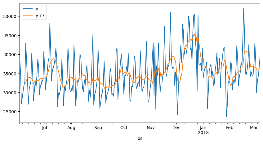
rolling：移動窓処理#

pandasのrollingで移動平均など取ることができます。
例えば直前7行の平均を各行求める場合、
df.rolling(7).mean()　といった形で使います。

直前N行だけでなく移動窓のとり方は色々設定可能です

https://pandas.pydata.org/docs/reference/api/pandas.DataFrame.rolling.html

import pandas as pd

# サンプルデータのロード
df = pd.read_csv("https://raw.githubusercontent.com/facebook/prophet/main/examples/example_pedestrians_covid.csv")
df["ds"]= pd.to_datetime(df["ds"])
df.set_index("ds",inplace=True)

df["y_r7"] = df["y"].rolling(7).mean()
df.head(10)

	y	y_r7
ds
2017-06-02	39230	NaN
2017-06-03	35290	NaN
2017-06-04	27083	NaN
2017-06-05	28727	NaN
2017-06-06	30315	NaN
2017-06-07	31947	NaN
2017-06-08	32678	32181.428571
2017-06-09	42988	32718.285714
2017-06-10	38413	33164.428571
2017-06-11	33640	34101.142857

df.head(280).plot(figsize=(10,5));

../_images/96eba92947b509d7dfe2e20ac0728a669e439e0bbf7cefa8c265b37eef97c9a1.png

melt pivot：縦持ち化、横持ち化#

pandas.DataFrameの meltメソッド、pivotメソッドで、縦持ち・横持ち変換ができます！

pivot https://pandas.pydata.org/pandas-docs/stable/reference/api/pandas.DataFrame.pivot.html

melt https://pandas.pydata.org/docs/reference/api/pandas.DataFrame.melt.html

import pandas as pd
import plotly.express as px

df = px.data.stocks()

df_long = df.melt(id_vars=['date'],
                  value_vars=['GOOG','AAPL','AMZN','FB','NFLX','MSFT'],
                  var_name='company',
                  value_name='stocks')
df_long

	date	company	stocks
0	2018-01-01	GOOG	1.000000
1	2018-01-08	GOOG	1.018172
2	2018-01-15	GOOG	1.032008
3	2018-01-22	GOOG	1.066783
4	2018-01-29	GOOG	1.008773
...	...	...	...
625	2019-12-02	MSFT	1.720717
626	2019-12-09	MSFT	1.752239
627	2019-12-16	MSFT	1.784896
628	2019-12-23	MSFT	1.802472
629	2019-12-30	MSFT	1.788185

630 rows × 3 columns

df_wide = df_long.pivot(index="date",columns="company",values="stocks")
df_wide

company	AAPL	AMZN	FB	GOOG	MSFT	NFLX
date
2018-01-01	1.000000	1.000000	1.000000	1.000000	1.000000	1.000000
2018-01-08	1.011943	1.061881	0.959968	1.018172	1.015988	1.053526
2018-01-15	1.019771	1.053240	0.970243	1.032008	1.020524	1.049860
2018-01-22	0.980057	1.140676	1.016858	1.066783	1.066561	1.307681
2018-01-29	0.917143	1.163374	1.018357	1.008773	1.040708	1.273537
...	...	...	...	...	...	...
2019-12-02	1.546914	1.425061	1.075997	1.216280	1.720717	1.463641
2019-12-09	1.572286	1.432660	1.038855	1.222821	1.752239	1.421496
2019-12-16	1.596800	1.453455	1.104094	1.224418	1.784896	1.604362
2019-12-23	1.656000	1.521226	1.113728	1.226504	1.802472	1.567170
2019-12-30	1.678000	1.503360	1.098475	1.213014	1.788185	1.540883

105 rows × 6 columns

以下の記事でpandasのデータの縦持ち・横持ち変換メソッドが図でまとめられていてわかりやすいと思いました。
URLはこちらです。
https://itdepends.hateblo.jp/entry/2020/02/25/220604

pivot, pivot_table, melt, stackは覚えておくとスムーズに集計できて便利だと思います。

rank：順位付け#

rankメソッドで数値の大小で順位付けができます。
ascending で昇順・降順を設定し、method で同値の処理方法を指定できます。

公式ドキュメント
https://pandas.pydata.org/docs/reference/api/pandas.DataFrame.rank.html

import pandas as pd
# サンプルデータ
df = pd.Series([41,55,68,75,75,80,92],name="val").to_frame()

df["val_asc_rank"] = df["val"].rank() # 小さい順でランク付け。同値は平均順位を返す
df["val_desc_rank"] = df["val"].rank(ascending=False) # 大きい順でランク付け。同値は平均順位を返す
df["val_desc_rank_min"] = df["val"].rank(ascending=False,method='min')  # 同値同士は小さい側(高ランク側)の順位で統一

df

	val	val_asc_rank	val_desc_rank	val_desc_rank_min
0	41	1.0	7.0	7.0
1	55	2.0	6.0	6.0
2	68	3.0	5.0	5.0
3	75	4.5	3.5	3.0
4	75	4.5	3.5	3.0
5	80	6.0	2.0	2.0
6	92	7.0	1.0	1.0

clip：上限下限を定め値の範囲を制限する#

clipメソッドで、指定した値の範囲になるようSeriesの値を変更できます。
指定した値以上or以下の値は、指定した値に置き換えられます。

公式ドキュメント
https://pandas.pydata.org/docs/reference/api/pandas.Series.clip.html#pandas.Series.clip

import pandas as pd
df = pd.Series([-4,-2,0,2,4,6,8,10,12,14],name='num').to_frame()
df["clipped_num"]=df["num"].clip(lower=0,upper=10) # 0以上10以下にする
df

	num	clipped_num
0	-4	0
1	-2	0
2	0	0
3	2	2
4	4	4
5	6	6
6	8	8
7	10	10
8	12	10
9	14	10

cut：数値データを区間分け#

pandas.cut を使うと、数値データを簡単に区間分けできます。
手動で if 文を書くよりスッキリ書けて便利です。
右端を含む/含まないも指定できるので、柔軟に使えます💡

公式ドキュメント
https://pandas.pydata.org/docs/reference/api/pandas.cut.html

例えば、次のように年齢の区分分けなどに使えます。

import pandas as pd
df = pd.Series([3,14,20,32,40,56,68,78,82,94],name='年齢').to_frame()

# 右側の値をそのカテゴリに含める場合 right=True
df["境界値"] = pd.cut(df["年齢"],bins=[0,20,40,60,80,100], right=True)
df["区分名"] = df["境界値"].map(lambda x:f"{x.left}超{x.right}以下")

# 右側の値をそのカテゴリに含めない場合 right=False
df["境界値R"] = pd.cut(df["年齢"],bins=[0,20,40,60,80,100],right=False)
df["区分名R"] = df["境界値R"].map(lambda x:f"{x.left}以上{x.right}未満")

# 事前にラベルを設定することも可能
df["年齢区分"] = pd.cut(df["年齢"],bins=[0,20,40,60,80,100],right=False,
                    labels=["未成年","若年層","中年層","高年層","超高年層"])

df

	年齢	境界値	区分名	境界値R	区分名R	年齢区分
0	3	(0, 20]	0超20以下	[0, 20)	0以上20未満	未成年
1	14	(0, 20]	0超20以下	[0, 20)	0以上20未満	未成年
2	20	(0, 20]	0超20以下	[20, 40)	20以上40未満	若年層
3	32	(20, 40]	20超40以下	[20, 40)	20以上40未満	若年層
4	40	(20, 40]	20超40以下	[40, 60)	40以上60未満	中年層
5	56	(40, 60]	40超60以下	[40, 60)	40以上60未満	中年層
6	68	(60, 80]	60超80以下	[60, 80)	60以上80未満	高年層
7	78	(60, 80]	60超80以下	[60, 80)	60以上80未満	高年層
8	82	(80, 100]	80超100以下	[80, 100)	80以上100未満	超高年層
9	94	(80, 100]	80超100以下	[80, 100)	80以上100未満	超高年層

json_normalize：入れ子jsonを使いやすく#

pd.json_normalizeで入れ子構造を持つjson形式のデータをフラットなDataFrameに変換することができます。
これを使えばjsonファイルが扱いやすくなると思います。

公式ドキュメント
https://pandas.pydata.org/docs/reference/api/pandas.json_normalize.html

data = [
    {
        "id": 1,
        "name": "Cole Volk",
        "fitness": {"height": 130, "weight": 60},
    },
    {
        "id": 2,
        "name": "Faye Raker",
        "fitness": {"height": 130, "weight": 60},
    },
]

pd.json_normalize(data)

	id	name	fitness.height	fitness.weight
0	1	Cole Volk	130	60
1	2	Faye Raker	130	60

pd.DataFrame(data)

	id	name	fitness
0	1	Cole Volk	{'height': 130, 'weight': 60}
1	2	Faye Raker	{'height': 130, 'weight': 60}

mapやapplyでtqdm：進捗がわかる#

tqdmはpandasのmap、applyに対しても利用できます。
最初に、tqdm.pandas()を実行すれば、それぞれprogress_map、progress_applyに置き換えるだけで、プログレスバーが出るようになります。

import pandas as pd
import numpy as np
from tqdm import tqdm

# pandasでtqdm使う場合はこれを実行しておく
tqdm.pandas()

# サンプルデータ
df = pd.DataFrame(np.random.rand(500000, 2), columns=["a","b"])

df["c"] = df["a"].progress_map(lambda x:x+1)

100%|██████████| 500000/500000 [00:00<00:00, 1113312.92it/s]

df["d"] = df.progress_apply(lambda x:x["a"]+x["b"], axis=1)

100%|██████████| 500000/500000 [00:04<00:00, 120643.85it/s]

%%time
# 補足：四則演算ならmapやapply使わずとも以下のように計算できる
df["c"] = df["a"]+1
df["d"] = df["a"]+df["b"]

CPU times: user 2.17 ms, sys: 7.95 ms, total: 10.1 ms
Wall time: 10.4 ms

.csv.gz：保存容量節約#

pandasのread_csvやto_csvは、gzip圧縮されたcsvファイル(.csv.gz)にもそのまま使うことができます。
ファイルサイズを節約できて便利です。
ただし、通常のcsvより少し時間がかかります。

import pandas as pd
import seaborn as sns
df = sns.load_dataset('iris')

df.to_csv("/content/data.csv.gz")
df.to_csv("/content/data.csv")  # 比較用

df = pd.read_csv("/content/data.csv.gz")

from pathlib import Path
# ファイルサイズ
print("csv：{:.2f}[kB]".format(Path("/content/data.csv").stat().st_size/(1024**1)))
print("csv.gz：{:.2f}[kB]".format(Path("/content/data.csv.gz").stat().st_size/(1024**1)))

csv：4.25[kB]
csv.gz：1.10[kB]

select_dtype：指定した型の列が取れる#

pandas DataFrameのselect_dtypesメソッドで、特定のdtypeを含む/含まない列群のDataFrameを抽出することができます。 dtypeごとに処理を分けたいときなどに便利です。

https://pandas.pydata.org/docs/reference/api/pandas.DataFrame.select_dtypes.html

import pandas as pd
import seaborn as sns

df = sns.load_dataset('titanic').head(5)
df

	survived	pclass	sex	age	sibsp	fare	embarked	class	who	adult_male	deck	embark_town	alive	alone
0	0	3	male	22.0	1	7.2500	S	Third	man	True	NaN	Southampton	no	False
1	1	1	female	38.0	1	71.2833	C	First	woman	False	C	Cherbourg	yes	False
2	1	3	female	26.0	0	7.9250	S	Third	woman	False	NaN	Southampton	yes	True
3	1	1	female	35.0	1	53.1000	S	First	woman	False	C	Southampton	yes	False
4	0	3	male	35.0	0	8.0500	S	Third	man	True	NaN	Southampton	no	True

df.select_dtypes(include='float')

	age	fare
0	22.0	7.2500
1	38.0	71.2833
2	26.0	7.9250
3	35.0	53.1000
4	35.0	8.0500

df.select_dtypes(exclude='float')

	survived	pclass	sex	sibsp	embarked	class	who	adult_male	deck	embark_town	alive	alone
0	0	3	male	1	S	Third	man	True	NaN	Southampton	no	False
1	1	1	female	1	C	First	woman	False	C	Cherbourg	yes	False
2	1	3	female	0	S	Third	woman	False	NaN	Southampton	yes	True
3	1	1	female	1	S	First	woman	False	C	Southampton	yes	False
4	0	3	male	0	S	Third	man	True	NaN	Southampton	no	True

filter：正規表現で行か列をフィルタリング#

filterメソッドを使うと、正規表現で行or列をフィルタリングできます。
列名に規則性があれば抽出が楽になり便利です。

公式ドキュメント
https://pandas.pydata.org/docs/reference/api/pandas.DataFrame.filter.html

import pandas as pd
# サンプルデータ
df = pd.DataFrame([[1,2,3,4,5],[1,2,3,4,5],[1,2,3,4,5]],
                  columns=["foo_a","foo_b","bar_a","bar_b","bar_c"])
df

	foo_a	foo_b	bar_a	bar_b	bar_c
0	1	2	3	4	5
1	1	2	3	4	5
2	1	2	3	4	5

# 例：列名がfoo_から始まる列に限定してデータフレームを取得
df.filter(regex="^foo_")

	foo_a	foo_b
0	1	2
1	1	2
2	1	2

ydata_profiling：データの全体像がざっくりわかる#

ydata-profiling(旧名称：pandas-profiling)を使うと、データの分布や欠損の有無などをまとめてHTML出力してくれます。最初にどんなデータかざっくり確認したいとき便利だと思います。

ydataai/ydata-profiling

!pip install ydata-profiling

from ydata_profiling import ProfileReport
import seaborn as sns
df = sns.load_dataset('iris') # サンプルデータ
profile = ProfileReport(df, title="Profiling Report")

Upgrade to ydata-sdk

Improve your data and profiling with ydata-sdk, featuring data quality scoring, redundancy detection, outlier identification, text validation, and synthetic data generation.

profile

  0%|          | 0/5 [00:00<?, ?it/s]
100%|██████████| 5/5 [00:00<00:00, 44.93it/s]

	sepal_length	sepal_width	petal_length	petal_width
0	5.1	3.5	1.4	0.2
1	4.9	3.0	1.4	0.2
2	4.7	3.2	1.3	0.2
3	4.6	3.1	1.5	0.2
4	5.0	3.6	1.4	0.2

	A	B	C	D
R0	A0	B0	C0	D0
R1	A1	B1	C1	D1
R2	A2	B2	C2	D2
R3	A3	B3	C3	D3
R4	A4	B4	C4	D4
R5	A5	B5	C5	D5
R6	A6	B6	C6	D6
R7	A7	B7	C7	D7

	A	B	C	D	E	F	G
R0	A0	B0	C0	D0	B2	D2	F2
R1	A1	B1	C1	D1	B3	D3	F3
R2	A2	B2	C2	D2	B6	D6	F6
R3	A3	B3	C3	D3	B7	D7	F7

	val	val_asc_rank	val_desc_rank	val_desc_rank_min
0	41	1.0	7.0	7.0
1	55	2.0	6.0	6.0
2	68	3.0	5.0	5.0
3	75	4.5	3.5	3.0
4	75	4.5	3.5	3.0
5	80	6.0	2.0	2.0
6	92	7.0	1.0	1.0

	sepal_length	sepal_width	petal_length	petal_width
0	5.1	3.5	1.4	0.2
1	4.9	3.0	1.4	0.2
2	4.7	3.2	1.3	0.2
3	4.6	3.1	1.5	0.2
4	5.0	3.6	1.4	0.2

	A	B	C	D
R0	A0	B0	C0	D0
R1	A1	B1	C1	D1
R2	A2	B2	C2	D2
R3	A3	B3	C3	D3
R4	A4	B4	C4	D4
R5	A5	B5	C5	D5
R6	A6	B6	C6	D6
R7	A7	B7	C7	D7

	A	B	C	D	E	F	G
R0	A0	B0	C0	D0	B2	D2	F2
R1	A1	B1	C1	D1	B3	D3	F3
R2	A2	B2	C2	D2	B6	D6	F6
R3	A3	B3	C3	D3	B7	D7	F7

	val	val_asc_rank	val_desc_rank	val_desc_rank_min
0	41	1.0	7.0	7.0
1	55	2.0	6.0	6.0
2	68	3.0	5.0	5.0
3	75	4.5	3.5	3.0
4	75	4.5	3.5	3.0
5	80	6.0	2.0	2.0
6	92	7.0	1.0	1.0

Pandas Tips Collection

Contents

Pandas Tips Collection#

基本的にDataFrameのメソッドはDataFrameのコピーを返す#

メソッドチェーン：きれいにコードが書ける#

query：簡単な条件指定方法#

display：表示方法の調整#

loc, iloc：範囲指定の注意点#

reindex：indexを再設定#

info：メモリ使用量などがわかる#

describe：基本統計#

explode：リストの列を展開#

concat , merge , join：結合方法の種類#

map：列の全値に同じ処理を適用#

apply：各行複数列使って、全行同じ処理を適用#

groupby：グループごとの集計#

groupby.count groupby.size：カウントの仕方の種類#

groupby(dropna=False,as_index=False)：便利オプション#

groupby.apply：任意の関数を適用#

groupby.transform：グループごとに同じ集計値を返す#

groupby.agg：複数種類の集約をいっぺんにできる#

pd.Grouper：日付のグループ集計に便利#

value_counts：値ごとにデータ数をカウント#

strアクセッサ：文字列操作を高速に#

str.replace：文字列の置換#

str.lower str.upper：小文字化、大文字化#

str.zfill：0埋め#

str.contains：その文字を含むか#

dtアクセッサ：日付から情報抽出#

intの欠損について#

欠損値補間#

rolling：移動窓処理#

melt pivot：縦持ち化、横持ち化#

rank：順位付け#

clip：上限下限を定め値の範囲を制限する#

cut：数値データを区間分け#

json_normalize：入れ子jsonを使いやすく#

mapやapplyでtqdm：進捗がわかる#

.csv.gz：保存容量節約#

select_dtype：指定した型の列が取れる#

filter：正規表現で行か列をフィルタリング#

ydata_profiling：データの全体像がざっくりわかる#

	sepal_length	sepal_width	petal_length	petal_width
0	5.1	3.5	1.4	0.2
1	4.9	3.0	1.4	0.2
2	4.7	3.2	1.3	0.2
3	4.6	3.1	1.5	0.2
4	5.0	3.6	1.4	0.2

	A	B	C	D
R0	A0	B0	C0	D0
R1	A1	B1	C1	D1
R2	A2	B2	C2	D2
R3	A3	B3	C3	D3
R4	A4	B4	C4	D4
R5	A5	B5	C5	D5
R6	A6	B6	C6	D6
R7	A7	B7	C7	D7

	A	B	C	D	E	F	G
R0	A0	B0	C0	D0	B2	D2	F2
R1	A1	B1	C1	D1	B3	D3	F3
R2	A2	B2	C2	D2	B6	D6	F6
R3	A3	B3	C3	D3	B7	D7	F7

	val	val_asc_rank	val_desc_rank	val_desc_rank_min
0	41	1.0	7.0	7.0
1	55	2.0	6.0	6.0
2	68	3.0	5.0	5.0
3	75	4.5	3.5	3.0
4	75	4.5	3.5	3.0
5	80	6.0	2.0	2.0
6	92	7.0	1.0	1.0